Topic model for incident detection, description and theoretical analysis (this material should be quite clear)

Description of the model

As I use citations in some part, here is the bibtex file

General

The derivation of the model and its approximation algorithm, and the discussion about the feature is based on multitude of different books, tutorials and articles EM algorithmh ,Mixture models and EM chapter 9, A. Ng mixture model and EM part 1 derivation,A. Ng mixture model and EM part 2 derivation.A. Ng explaining this on a video Each idea and description proposed is mostly a mixture of ideas derived from different sources.

The specific formulas for training the incident detection model and performing incident detection are given in Kinoshita et al. A Latent Dirichlet Allocation (LDA) equivalent method is used for modeling the traffic. First of all, the implemented method divides all the roads in Hong Kong into \texttt{S} segments. A segment is specified as a certain section of a route during a certain period of time. Next, speed observations obtained from GPS and road sensor data are used to train a traffic model. The result of the training will be \texttt{K} global traffic states distributed in each segment according to the segment’s local parameters. After the training of the model, each new observation is compared to the prior historical distribution in the segment using divergence functions.

Definitions

• S - number of segments
• K - number of traffic states
• N - number of speed observations
• Z - latent random variable - binary vector with ones and zeros and K elements (only one element = 1)
• X - observed random variable - scalar value, a speed observation in this case. (could be extended to be a vector)

Topic Modeling Theory

The topic model fitted on the traffic data in the article Kinoshita et al. \cite{kinoshita2015real} is derived from a probabilistic topic modeling technique. Topic modeling with latent variable mixture models is a broadly covered field in literature and has numerous applications in textual analysis, traffic modeling and genetic engineering. \cite{wang2011collaborative}´ \cite{chen2010probabilistic}´ \cite{yuan2012discovering}

The mixture of different models with latent variable parameters was first proposed by Blei et al. \cite{blei2003latent} in a paper describing Latent Dirichlet Allocation.

The aim of this methodology is to classify observations into topics. To do this, a generative probabilistic process is assumed to exist behind every observation. That means every observable observation is drawn from a certain latent random variable distribution or distributions. The goal is to reverse this process by inferring these latent random variables from the observed data.

Model Behind each observation:

In the generative model, every random variable except for the observation is considered to be latent. First, for each segment,

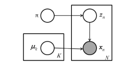
• a random variable Z (binary vector with only 1 element = 1) is drawn from a multinomial distribution which is dependent on parameter $\pi$. The multinomial distribution represents the probability over K different global traffic states in segment \texttt{S}
• based on the drawn Z, an observation is generated from the Poisson distribution specified by Z. Each Poisson distribution over speeds is dependent on a global parameter $\mu$

This process can be visualised with a simple graphical model shown on Figure \ref{graph_model}. Equivalently this model also means that every segment is considered as a mixture of traffic states which by themselves are distributions, thus every segment is a mixture model.

The graphical model for speed observation generation. The observed elements are shown in gray

The likelihood function for observations of speed-values for the entire set of observed data is given by the following equation:

$$L(\mu, \pi; X)=\prod_{1}^{S} \prod_{1}^{N_{s}} \sum_{1}^{K}p(x_{sn} \vert \mu_{k})p(\pi_{sk})$$

It can be interpreted as: For each road segment, for each observation, what is the combined likelihood of drawing observations X with parameters $\mu$ and $\pi$.

There are two significant parameters in this model. The local segment parameter $\pi$, which affects how traffic states are distributed in each segment, and the traffic state parameter $\mu$ for each of the K traffic states. Having established this generative model to the data, there exist multiple techniques to optimise the parameters of this model to the data. It is important to make a difference between the random variables (X -observed , Z-latent) and the point estimated parameters ($\mu$ and $\pi$).

Bayes background

Theoretically the most straightforward approach to infer the parameters from the observed data is to use Bayesian inference. This can be thought of as reversing the generative process.

\textbf{General Example of Bayes formula in probability Theory} $P(A \vert B)=\frac{P(B \vert A)P(A)}{\sum{P(B|A)P(A)}}$

In Bayesian inference, It is supposed that there is a distribution over the latent random variables and data is fixed. The main aim of Bayesian rule is thus to calculate the probability of parameter/s based on the given data. It is often done incrementally, i.e. through improving/deepening the belief in certain parameters/ infered latent variable as the amount of data “going through” the calculations grows. $\stackrel{\text{Posterior}}{P(\theta \vert data)}=\frac{\stackrel{\text{Likelihood}}{P(data \vert \theta)} \stackrel{\text{Prior}}{P(\theta)}}{\stackrel{\text{Marginal}}{P(data)} }$

All the elements in the above formula are dependent on a chosen model. The model becomes important for the margin to explain what the probability of data is. It is the probability of the data based on the model and chosen parameters.
Here, the Bayesian approach would also theoretically work out. To do that, it would be necessary to consider the parameters $\mu$ and $\pi$ in addition to the segment distribution variable Z as random variables. The general application of the Bayes formula in this case would look like this
$p(\theta, Z | x) = \frac{p(\theta, z, x )}{p(x)}$ In this formula $\theta$ is considered as the set of all parameters an $Z$ is considered as latent random variables which show the cluster of or class of the observation (e.g. which Poisson distribution generated the observation). The likelihood of the data in the above formula’s denominator which is also considered the normalising factor or the marginal becomes intractable to compute in real life with more complex models. Thus approximation methods like the Variational inference or Monte Carlo sampling should be used \cite{blei2003latent}. In this case a more simple approximation was chosen in the face of the Expectization Maximization (EM) algorithm. This method resembles more the variational inference based methods but only gives point estimates to the parameters $\mu$ and $\pi$.

Approximation Methodology

The goal for the used EM algorithm is simply to give a point estimate for the parameters $\mu$ and $\pi$ from the observations so $p(x)$. The straight log-likelihood maximisation for the parameters $p(X \mid \theta)=\sum^{N}_{i=1}{log p(x,\theta)}$ is difficult because of all the possible classes each observation could come from. However the nature of the above-presented model allows to divide the parameter estimation into two steps. More explicitly we can repeatedly construct a lower-bound on the log-likelihood function (E-step), and then optimise that lower-bound (M-step). This approach follows the logic of the EM algorithm. The exact formulas for approximation in the E-step and M-step are brought out in the method-proposing paper and are left out from this dissertation for the sake of clarity. The general idea for the approximation goes like this: First ther is the E-step. In this step, the Expectation for the complete dataset (X,Z) is calculated. To do that, the posterior probability of Z given X is calculated. This can be seen as the responsibility that component k takes for ‘explaining’ the observation x. The calculated posterior probability for Z used in a specific combination with the parameters likelihood allows through the usage of Jensen’s equality to derive a lower bound for the likelihood function. This lower bound can then maximized in the M-step. Going iteratively through E-step and M-step monotonically increases the likelihood function.

Detecting Anomalies

After the parameters have been inferred globally and for each of the segments, new observations will be compared with the historical data based model. To do that, Bayesian inference is used again inside a specific time window to build a new distribution for the specific local segments using again the global traffic state parameters. Then the new posterior distribution is compared with the old distribution using weighted KL divergence.

Analysis of The Model

Parameters to Random Variables

Currently the proposed model estimates the parameters in all the locations as point estimates. Although the exact estimation of parameters gives the same results as when considering the parameters as random variables coming from distributions, it does not give the ability to assess the strengths of predictions in each of the segments. This is without a reason because a lot of authors have proposed methods how to integrate parameter inference to the EM algorithm \cite{emgupta}´ \cite{bishop2006pattern}. In addition, the predicition capabilities could also be assessed using regular statistical reliability methods like p-value and trust intervals to give information on how trustworthy each assessment is based on the underlying data. Addition of parameter assessment can be used to further develop the Hong Kong traffic monitoring system to take advantage of traffic monitoring using probabalistic graphs and source to target queries on top of such graphs \cite{hua2010probabilistic}.

Poisson to Gaussian

Essentially when speed observations are the only input to the model, the training deals with finding an average $\lambda$ for each of the K traffic states and then mixing these averages together on each road. Based on that, the choice of Poisson distribution is suprising because it is distribution which gives a probability to a number of occurences of a specific situation, not the probability of the occurence itself. Here a Gaussian distribution with two parameters instead of one for the Poisson distribution would be naturally more suitable because for such data the standard deviation is also an important consideration.This is what the Poisson Mixture model completely misses. Using Gaussian Mixtures together with the EM algorithm is a standard pratice in machine learning and both point estimate and inference methods have been developed for it \cite{emgupta}´ \cite{ngemalgo}.

Start modeling anomalies

The methods in traffic accident detection can broadly be divided into rule-based methods: methods which have defined the characteristics of traffic accidents manually \cite{wang2013hybrid}´ \cite{LDA_SOCIAL}´ \cite{kinoshita2015real} an methods which try to use supervised learning to differ traffic accidents based on some chosen features \cite{wang2013hybrid}´ \cite{srinivasan2005adaptive}´ \cite{jin2001classification}. In addition , methods have been developed which statistically model a normal condition for traffic and perform anomaly detection \cite{HMM_SOCIAL}´. The method used in this dissertation falls into the third category method of modeling a normal traffic state from which anomalies are detected. Although this method is aimed at modeling a normal traffic state for each of the road segments, it fails to model traffic accidents information as its purpose is only to detect divergence from that modeled normal state. Considering for example that in Hong Kong there happened 14,000 accidents in a year, this is done without justification as traffic accident patterns could provide the model with valuable information. Considering that using speedpanels it was possible to obtain around 14 thousand accident records for 3 thousand accidents, addition of an accident model to this algorithm can prove to be useful. The current model only takes into account the traffic state in a certain time and does not consider the traffic state change into its model. The sudden change of traffic definitely is a likely indicator of a traffic accident which this model completely misses. Wang et al. has proposed a Neural Network and Time Series Analysis based solution which models traffic accidents and also takes into account the time factor. That solution has only been tested using loop detectors and has not shown AUC values in their results. Overall, based on the quantity and divergence of methods performing incident detection in the literature, and a lack of papers comparing the results on one specific dataset, the author of this dissertation strongly feels that an experimental study comparing the latest state-of-the-art methods for incident detection on one dataset could proce to be very useful.

More features

Topic modeling is based on co-ccurence of observations in certain clusters. In Natural Language Processing (NLP), LDA model assumes a co-occurrence of similar words on one specific topic and assigns for each word a topic based on systematic co-occurences. It is possible to easily analyse whether the classified topics actually are good or not based on the words inside the topics. If the words “pollution” and “playground” have been classified to act together we can clearly say that it is not performing well. An example of good co-occurence is the words “marine” and “pollution” co-occuring in a topic. For NLP this kind of extra grouping of words to topics is more important because the words do not have a natural linear numerical basis to be grouped together. Speed observations however are already grouped together on a numerical scale. It is more likely that observations 71 and 72 occur together than 71 and 10. Considering the capapility of the LDA, however, extending this model to using multiple features could improve the model with less simplistic connections by creating traffic states based on non-linear features. Such extra information could be useful for cases like in Hong Kong, where the dataset is relatively small. The addition of extra traffic features has been proposed by Kinoshita et al. in their paper but they have not implemented the solution for this.